Secondary Axis

Quantities that share the reaction coordinate but not the units - bond lengths against energy, say - can be drawn on a right-hand y-axis by passing secondary to plot().

It takes a dict of {label: [values]} on the same x-indices as the primary series, folded into the same legend. Set y2={'label': ...} so the right-hand scale says what it is.

plotter = ReactionProfilePlotter(
    figsize=(7.6, 4),
    curviness=0.0,
    labels=False,
    energy="E",
    square=True,
    x_label="reaction coordinate  λ",
    legend={"outside": True, "anchor": 1.22},
    y2={"label": "bond length (Å)", "colors": "plasma"},
)
plotter.plot(
    {"force field": [0.0, 5.2, 12.4, 3.1, -1.2], "g-xTB": [0.0, 4.4, 10.9, 2.0, -2.5]},
    secondary={
        "C1-O3 (breaking)": [1.43, 1.62, 2.10, 2.85, 3.30],
        "C1-O14 (forming)": [3.20, 2.75, 2.05, 1.55, 1.42],
    },
    filename="../images/profile24",
)

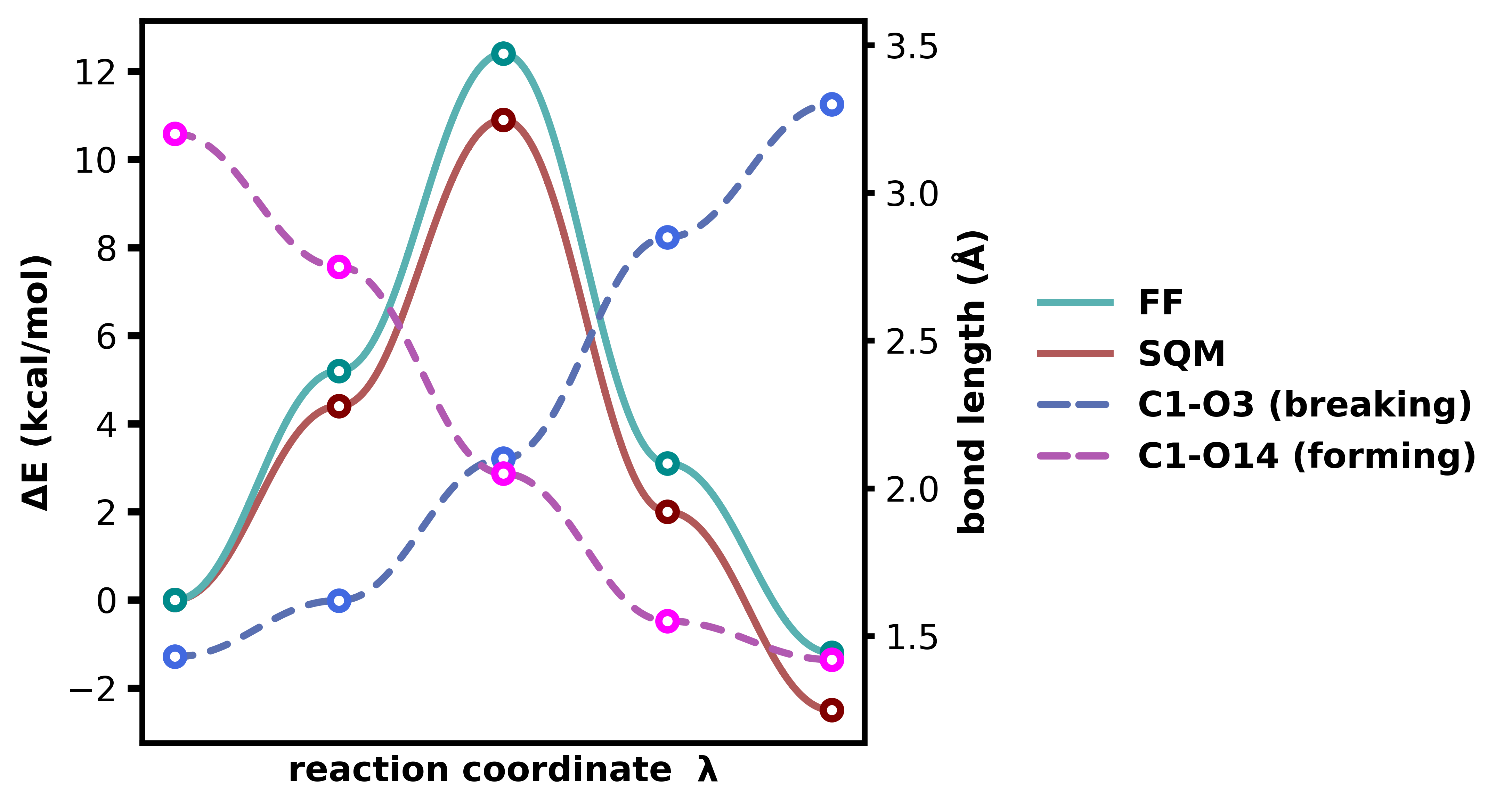
Styling the two axes

A style key set on the plotter applies to both axes. The same key inside y2 overrides it for the right-hand axis alone, so the two can be styled independently:

ReactionProfilePlotter(
    curviness=0.0,
    point_type="bar",                 # both axes
    y2={
        "point_type": "dot",          # right-hand axis only
        "curviness": 0.42,
        "colors": "plasma",
        "linestyle": "solid",
        "desaturate": False,
    },
)

Any of colors, curviness, line_width, marker_size, point_type, bar_length, bar_width, connect_bar_ends, desaturate, desaturate_factor and dash_spacing can go in y2, plus two of its own: label for the right-hand axis label, and linestyle, which defaults to '--' here so the second scale reads as separate. Set 'solid', or any matplotlib spec - see Plotting Customisation.

Legend

The legend dict is passed straight to matplotlib’s legend(), plus outside and anchor. With a secondary axis, anchor needs about 1.22 to clear the right-hand axis and its label; square=True then stops the axes being squashed to make room. See Plotting Customisation for the full set.

Note

axes governs the secondary axis too: axes='None' draws no right-hand spine or ticks.